

- Transfer Function Definition: A transfer function is defined as the ratio of the Laplace transform of a system’s output to the input, assuming initial conditions are zero.
- Utilization of Block Diagrams: Block diagrams simplify complex control systems into manageable components, making it easier to analyze and derive transfer functions.
- Understanding Poles and Zeros: Poles and zeros critically influence a system’s behavior by indicating points where the transfer function respectively becomes infinite or zero.
- Laplace Transform in Control Systems: Laplace transform is essential for representing all types of signals in a uniform format, aiding in the mathematical analysis of control systems.
- Impulse Response Insight: The output from an impulse input reveals the transfer function, illustrating the direct relationship between a system’s input and output.
A transfer function represents the relationship between the output signal of a control system and the input signal, for all possible input values. A block diagram is a visualization of the control system which uses blocks to represent the transfer function, and arrows which represent the various input and output signals.
Every control system has a reference input, often called excitation or cause, that works through a transfer function to create a controlled output or response.
Thus the cause and effect relationship between the output and input is related to each other through a transfer function.
In a Laplace Transform, if the input is represented by R(s) and the output is represented by C(s), then the transfer function will be:
That is, the transfer function of the system multiplied by the input function gives the output function of the system.
What is a Transfer Function
Transfer Function Explained: It is defined as the ratio of the Laplace transform of the output to the Laplace transform of the input, assuming zero initial conditions.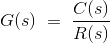
Procedure for determining the transfer function of a control system are as follows:
- We form the equations for the system.
- Now we take Laplace transform of the system equations, assuming initial conditions as zero.
- Specify system output and input.
- Lastly we take the ratio of the Laplace transform of the output and the Laplace transform of the input which is the required transfer function.
Inputs and outputs in a control system may differ. For instance, electric motors take electrical signals as inputs and produce mechanical outputs to rotate, while generators take mechanical inputs to generate electrical outputs.
But for mathematical analysis, of a system all kinds of signals should be represented in a similar form. This is done by transforming all kinds of signal to their Laplace form. Also the transfer function of a system is represented by Laplace form by dividing output Laplace transfer function to input Laplace transfer function. Hence a basic block diagram of a control system can be represented as

Where r(t) and c(t) are time domain function of input and output signal respectively.
Methods of Obtaining a Transfer Function
There are major two ways of obtaining a transfer function for the control system. The ways are:
- Block Diagram Method: It is not convenient to derive a complete transfer function for a complex control system. Therefore the transfer function of each element of a control system is represented by a block diagram. Block diagram reduction techniques are applied to obtain the desired transfer function.
- Signal Flow Graphs: The modified form of a block diagram is a signal flow graph. Block diagrams visually outline a control system, while signal flow graphs provide a more compact representation.
Poles and Zeros of Transfer Function
Generally, a function can be represented to its polynomial form. For example,
Now similarly transfer function of a control system can also be represented as
Where K is known as the gain factor of the transfer function.
Now in the above function if s = z1, or s = z2, or s = z3,….s = zn, the value of transfer function becomes zero. These z1, z2, z3,….zn, are roots of the numerator polynomial. As for these roots the numerator polynomial, the transfer function becomes zero, these roots are called zeros of the transfer function.
Now, if s = p1, or s = p2, or s = p3,….s = pm, the value of transfer function becomes infinite. Thus the roots of denominator are called the poles of the function.
Let’s represent the transfer function in its polynomial form:
Now, let us consider s approaches to infinity as the roots are all finite number, they can be ignored compared to the infinite s. Therefore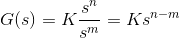
Hence, when s → ∞ and n > m, the function will have also value of infinity, that means the transfer function has poles at infinite s, and the multiplicity or order of such pole is n – m.
Again, when s → ∞ and n < m, the transfer function will have value of zero that means the transfer function has zeros at infinite s, and the multiplicity or order of such zeros is m – n.
Concept of Transfer Function
The transfer function is generally expressed in Laplace Transform and it is nothing but the relation between input and output of a system. Let us consider a system consists of a series connected resistance (R) and inductance (L) across a voltage source (V).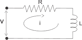
In this circuit, the current ‘i’ is the response due to applied voltage (V) as cause. Hence the voltage and current of the circuit can be considered as input and output of the system respectively.
From the circuit, we get,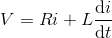
Now applying Laplace Transform, we get,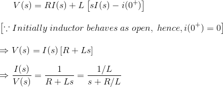
The transfer function of the system, G(s) = I(s)/V(s), the ratio of output to input.
1) Let us explain the concept of poles and zeros of transfer function through an example.
Solution
The zeros of the function are, -1, -2 and the poles of the functions are -3, -4, -5, -2 + 4j, -2 – 4j.
Here n = 2 and m = 5, as n < m and m – n = 3, the function will have 3 zeros at s → ∞. The poles and zeros are plotted in the figure below 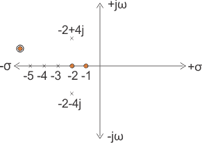
2) Let us take another example of transfer function of control system
Solution
In the above transfer function, if the value of numerator is zero, then
These are the location of zeros of the function.
Similarly, in the above transfer function, if the value of denominator is zero, then
These are the location of poles of the function.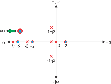
As the number of zeros should be equal to number of poles, the remaining three zeros are located at s →∞.
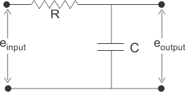
Example of Transfer Function of a Network
3)
Solution
In the above network it is obvious that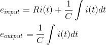
Let us assume,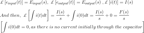
Taking the Laplace transform of above equations with considering the initial condition as zero, we get,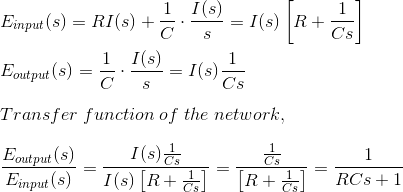
The Effect of Impulse Signal
The unit impulse signal is defined as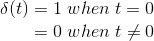

Laplace transform of unit impulse function is 1.
Now if input signal is unit impulse signal then,
The output function is same as its transfer function.
Transfer Function Example
1) The impulse response of a system is
What will be the transfer function of the system?
Solution
For impulse response, the output C(s) of the system is equal to transfer function of the system.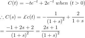
Therefore, transfer function of the system is
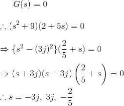
2) Find the poles and zeros of the function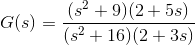
Solution
3) The poles and zeros are plotted on the is plain as shown below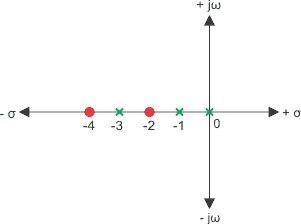
Find the transfer function.
Solution
Here, the poles are s = – 3, – 1, 0.
Therefore, denominator of the function would be,
the zeros are, -4, – 2.
Therefore, numerator of the function would be,
Therefore, transfer function would be,
Where, K is the gain factor of the control system.
4) Find the gain factor K of a transfer function whose value is 2 at s = 2 and the transfer function is given as
Solution
Now, as per condition of the problem,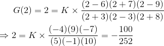
5) Find the transfer function of the following network.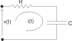
Solution
From the circuit we get,
Now applying Laplace transformation at both sides we get,
As the applied voltage is cause and the corresponding charging current is the effect, the applied voltage can be considered as input and charging current can be considered as output.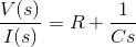
6) Find the transfer function of the network given below,
Solution
In the above figure, the input is applied voltage v(t) and the output is measured as the voltage appears across the capacitor C that is vc(t).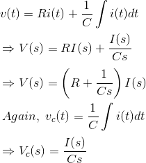
Laplace transformation of the transfer function is
7) A shaft of innertia J is rotated for an angle θ due to applied torque T against a bearing friction f. Find the transfer function of the system.
Solution
The differential equation form of the above statement is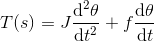
Taking Laplace transformation of both sides of the system,
As the applied torque is input and the output angular displacement is output of the system.
8) The impulse response of the system is given by c(t) = 1 – te-2t + sin3t. Find that transfer function of the system
Solution
9) Find the transfer function of the impulse response of a system given by
Solution


