High Pass Filter: Circuit, Transfer Function & Bode Plot

💡

Key learnings:

High Pass Filter Definition: A high pass filter allows frequencies higher than a certain cutoff and blocks lower ones, useful in electronic filtering.
Circuit Components: These filters can use simple components like resistors and capacitors or include operational amplifiers for more complex applications.
High Pass Filter Transfer Function: The transfer function mathematically represents how the filter processes signals, emphasizing frequencies above the cutoff.
Bode Plot Overview: A Bode plot visualizes the frequency response of the filter, showing changes in signal magnitude and phase with frequency.
Practical Applications: High pass filters are used in diverse fields like audio technology and image processing to enhance signal quality.

An electrical filter changes a signal according to frequency. It passes some frequency components with relatively little loss and attenuates others. The transition is gradual in every realizable filter.

Analog filters can use resistors, inductors, capacitors and amplifiers. Their component values and topology set the gain and phase response as a function of frequency.

A cut-off frequency defines an edge of a passband or stopband. For the first-order RC filter discussed below, the magnitude at this frequency is 1/√2 of the high-frequency gain, or about -3 dB. Other filter families can define their band edge and -3 dB point differently.

What is a High Pass Filter?

A high pass filter, also called a low-cut filter or bass-cut filter, attenuates low-frequency and DC components while passing higher-frequency components within its designed passband. “Pass” does not mean zero loss, and “attenuate” does not mean complete rejection.

A low-pass filter has the complementary frequency-selective role: it passes a low-frequency band and increasingly attenuates higher frequencies. The band pass filters in this family pass a band between lower and upper cutoff regions. None of these practical filters changes gain abruptly at one frequency.

High Pass vs Low Pass Filters

High-pass and low-pass responses are complementary concepts, but their practical circuits and uses are not exact opposites:

Types of High Pass Filters

There are many types of high-pass filters according to the circuit design and components used to make a filter. The various types of high-pass filters include:

Passive High Pass Filter

A passive filter uses resistors, capacitors and inductors without an active gain element. It needs no separate supply for amplification, but source and load impedances affect its response and passive losses can reduce signal amplitude.

A first-order passive high-pass circuit can use an RC network with output across the resistor or an RL network with output across the inductor. Higher-order passive designs can also use multiple reactive elements.

Active High Pass Filter

An active filter combines frequency-selective resistors and capacitors with an active device such as an operational amplifier. The active stage can provide gain. It can also buffer one section from another and reduce output impedance.

Common op-amp high-pass topologies include inverting first-order stages, Sallen-Key stages and multiple-feedback stages. The op amp’s gain-bandwidth, slew rate, noise and output range limit the useful frequency and signal range.

RC High Pass Filter

The basic passive RC high-pass filter places a capacitor in series with the input and a resistor to the reference node, with output measured across the resistor.

In the simple voltage-divider forms, interchanging the resistor and capacitor changes whether output is taken across the resistor for high-pass response or across the capacitor for low-pass response. The RC high-pass circuit is shown below.

Capacitive reactance increases as frequency decreases. At frequencies far below cutoff, the capacitor approaches an open circuit relative to the resistor, so little output appears across the resistor.

Capacitive reactance decreases as frequency increases. At frequencies far above cutoff, the capacitor approaches a short circuit relative to the resistor and the output approaches the input, subject to source and load impedance.

First Order High Pass Filter

A first-order high-pass filter has one pole in its transfer function. A passive RC or RL example contains one independent energy-storage element.

After common factors are removed, the transfer-function denominator has degree one in the Laplace variable ‘s’. Circuit order depends on independent stored-energy states, not simply on counting every capacitor and inductor symbol.

A first-order filter can be passive or active. An active RC version still needs frequency-selective passive components as well as its amplifier. The basic RC high-pass network is a first-order passive filter.

Second Order High Pass Filter

A second-order high-pass transfer function has two poles. It can be realised with a designed two-pole topology or by cascading two first-order sections. Unbuffered passive sections load each other, so their combined response cannot always be calculated as two isolated stages.

Far into the stopband, an ideal all-pole first-order high-pass section rises at 20 dB per decade and a second-order response rises at 40 dB per decade. Near cutoff, pole Q and response family also determine the curve.

Frequency Response of High Pass Filter — Pass Band and Stop Band for First Order and Second Order Filters

For example, the asymptotic stopband slopes are +20 dB/decade for a first-order Butterworth response and +40 dB/decade for a second-order Butterworth response.

Butterworth High Pass Filter

A Butterworth response is maximally flat in magnitude at the passband reference frequency and has no passband ripple. Its transition is less steep than an equal-order Chebyshev response. The figure below shows first-order and second-order high-pass examples.

Circuit Diagram and Frequency Response of Butterworth Filter

Chebyshev High Pass Filter

A Chebyshev response accepts equiripple error in one band to obtain a sharper transition than an equal-order Butterworth response. Type I has equiripple magnitude in the passband. Type II, or inverse Chebyshev, has a monotonic passband and equiripple stopband.

Chebyshev order and ripple are design choices based on passband tolerance and required attenuation. As Type I ripple approaches 0%, its response approaches the Butterworth case. Ripple is commonly specified in decibels; 0.5% is not the same specification as 0.5 dB, and neither is a universal choice. The figure compares representative Butterworth and Chebyshev responses.

Frequency Response Compression of Butterworth and Chebyshev High Pass Filter

A Type I Chebyshev filter places equal ripple in the passband and remains monotonic in the stopband. A Type II inverse Chebyshev filter remains monotonic in the passband and places equal ripple, with transmission zeros, in the stopband.

An elliptic, or Cauer, response permits ripple in both passband and stopband and adds transmission zeros. For a given order and ripple limits, it can provide a narrower transition than Butterworth or Chebyshev responses, with greater phase and transient distortion.

Bessel Filter

Butterworth prioritises a flat magnitude response. Chebyshev prioritises a sharper magnitude transition for a given order at the cost of ripple and usually more ringing or phase nonlinearity.

A Bessel response prioritises linear phase and maximally flat group delay near its reference frequency, giving low waveform distortion and overshoot. Its magnitude transition is slower than an equal-order Butterworth or Chebyshev response. Group delay is not exactly constant across an unlimited passband.

Passive vs Active High Pass Filter

According to the components used in the circuit, filters are classified into two types; Active Filter and Passive Filter.

	Active Filter	Passive Filter
Circuit elements	An active filter uses an amplifier such as an op amp or Transistor.	A passive filter uses resistors, capacitors or inductors without an active gain device.
Extra power supply	Its active devices require a power supply.	It needs no separate supply, but it draws energy from the signal source.
Frequency limitation	Its amplifier sets gain-bandwidth, slew-rate and signal-range limits.	Its components, parasitics, source and load also impose frequency limits.
Cost	Cost depends on the amplifier and precision components.	Cost depends on inductors, capacitors, power level and tolerances.
Stability	Stability depends on topology, amplifier and layout.	It cannot oscillate from active feedback, but loading and parasitics alter response.
Weight	Often low for RC op-amp circuits.	RC networks can be light; high-power inductors can be heavy.
Sensitivity	Sensitivity depends on topology, Q, tolerances and amplifier variation.	Sensitivity depends on topology, Q, loading and component tolerances.
Q Factor	The achievable Q can be high but remains topology- and amplifier-dependent.	Passive RLC networks can also achieve high Q with low-loss components.
Design	It needs biasing and amplifier checks, but many standard topologies are simple.	Simple RC filters are easy; loaded or high-Q LC designs require full network analysis.
Efficiency	There is no universal efficiency ranking; quiescent and signal power both matter.	Insertion loss and impedance matching determine passive power transfer.
Frequency Response Characteristic	Response sharpness is set by order, Q and approximation.	Passive filters can also realise sharp high-order responses.

High Pass Filter Transfer Function Equation

A transfer function describes the ratio of output to input in the Laplace domain for a linear time-invariant circuit under stated initial conditions. Substituting s = jω gives the sinusoidal steady-state frequency response.

The transfer function of a first order high pass filter is derived in the below equations.

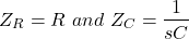
$\begin{align*} Z_R = R \,\, and \,\, Z_C = \frac{1}{sC} \end{align*}$

For the unloaded voltage-divider derivation, the output-element impedance is:

$\begin{align*} Z_O_u_t = Z_R \end{align*}$

The total series impedance seen by the ideal source is:

$\begin{align*} Z_I_n = Z_R + Z_C \end{align*}$

The transfer function is the output-voltage to input-voltage ratio. This derivation assumes zero source impedance and no external load across the resistor.

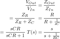
$\begin{align*} \begin{split} \frac{V_O_u_t}{V_I_n} &= \frac{Z_O_u_t}{Z_I_n} \ &= \frac{Z_R}{Z_R+Z_C} \ &= \frac{R}{R+\frac{1}{sC}} \ &= \frac{sCR}{sCR+1} \ T(s) &= \frac{s}{s+\frac{1}{RC}} \end{split} \end{align*}$

A first-order high-pass form with high-frequency gain a1 is:

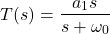
$\begin{align*} T(s) = \frac{a_1s}{s+\omega_0} \end{align*}$

Where:

$\begin{align*} a_1 = Amplitude \, of \, signal \end{align*}$

$\begin{align*} \omega_0 = Angular \, cutoff \, Frequency \end{align*}$

In the protected legacy formula above, a1 should be read as the dimensionless high-frequency gain, not the amplitude of a signal. At high frequency:

$\begin{align*} T ( s \to \infty) = a_1 \end{align*}$

At low frequency:

$\begin{align*} T ( s \to 0) = 0 \end{align*}$

The ideal first-order model therefore approaches zero gain at DC and approaches a1 at high frequency. A real active circuit eventually rolls off again because its amplifier has finite bandwidth.

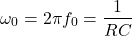
$\begin{align*} \omega_0 = 2\pi f_0 = \frac{1}{RC}\end{align*}$

$\begin{align*} Cutoff \, frequency \, \, \, f_0 = \frac{1}{2\pi RC}\end{align*}$

Cutoff Frequency High Pass Filter

Cutoff is a stated band-edge convention rather than a physical wall. For the first-order RC response, the cutoff is the -3 dB point where output magnitude is 1/√2 of its asymptotic passband value.

Above cutoff, gain approaches the high-frequency passband value. Below cutoff, attenuation increases as frequency falls. The output remains finite except at DC in the ideal model.

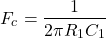
The designer chooses R and C to place the first-order RC pole at the required frequency. The same pole-frequency expression applies to the simple RC high-pass and low-pass voltage dividers.

$\begin{align*} F_c = \frac{1}{2\pi R C} \end{align*}$

For certain buffered or active two-section topologies, both resistor-capacitor products determine the natural frequency shown below. This is not a universal -3 dB cutoff formula for any two unbuffered RC sections because loading and pole Q matter.

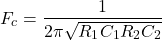
$\begin{align*} F_c = \frac{1}{2\pi \sqrt{R_1 C_1 R_2 C_2}} \end{align*}$

If R1 equals R2 and C1 equals C2 under the assumptions of that topology, the natural-frequency expression reduces to:

$\begin{align*} F_c = \frac{1}{2\pi R_1 C_1} \end{align*}$

High Pass Filter Bode Plot or Frequency Response

A bode plot shows magnitude in decibels and phase in degrees against logarithmic frequency. A first-order high-pass response has a zero at the origin and one pole, while its low-pass counterpart has no zero at the origin.

Set s = jω in the transfer function to calculate the magnitude and phase curves shown below.

For unity high-frequency gain, the magnitude is:

$\begin{align*} | H(j \omega)|= \frac{\omega}{\sqrt{\omega^2 + (\frac{1}{RC})^2}} \end{align*}$

The phase is 90° minus arctan(ωRC). The protected legacy equation below intends arctan even though its inverse-tangent typesetting is malformed.

$\begin{align*} \theta(j\omega) = 90^\circ - \tan^-^1(\omega RC) \end{align*}$

Magnitude Plot

Far below cutoff, the first-order magnitude rises at approximately +20 dB per decade as frequency increases. A stopband is defined by the required attenuation, not automatically by every frequency below cutoff.

Above the transition region, the response approaches its passband gain. A design specification states the passband edge and allowed ripple or loss.

At the first-order RC cutoff, output magnitude is 1/√2, or about 70.7%, of the asymptotic high-frequency output, corresponding to -3.01 dB in power-ratio convention.

Phase Plot

At the first-order RC cutoff, output leads input by +45 degrees. The ideal mathematical response approaches constant gain as frequency tends to infinity, but every physical component has parasitic effects and every active device has finite bandwidth.

The op amp, capacitor dielectric, resistor parasitics, circuit layout, source and load set the real upper-frequency limit.

Ideal High Pass Filter

An ideal high-pass model has zero magnitude below the cutoff and unit magnitude above it, with an instantaneous transition. Such a response is non-causal and cannot be realised exactly.

The ideal magnitude response below assumes unity passband gain. It keeps the magnitude of components above cutoff and removes those below cutoff. The sharp discontinuity would require an unrealizable infinite-order response.

The ideal magnitude is expressed piecewise below. In the second condition, the intended expression is |ω| < ωc; the opening absolute-value bar is missing from the protected legacy formula.

$\begin{equation*} |H(\omega)| = \begin{cases} 1, & |\omega|>\omega_c \\ 0, & \omega|<\omega_c \end{equation*}$

The frequency response characteristics of an ideal high pass filter is as shown in below figure.

No practical filter has this ideal discontinuity. A Butterworth response offers a ripple-free passband, but whether it is closer to the required response than Chebyshev, elliptic or Bessel depends on magnitude, phase, delay and transient specifications.

Applications of High Pass Filters

The applications of high pass filters include:

Audio equipment uses it for AC coupling, rumble removal, crossover networks and protection against unwanted subsonic content.
Image processing uses two-dimensional high-pass kernels to detect edges and fine spatial detail, while also amplifying high-spatial-frequency noise.
Sensor and control systems use high-pass stages to remove offsets, isolate changing components or implement lead and derivative-like behaviour within a limited band.

	High Pass Filter (HPF)	Low Pass Filter (LPF)
Definition	An HPF attenuates low frequencies and passes a higher-frequency band. Also called a low-cut filter.	An LPF passes a lower-frequency band and attenuates higher frequencies. Also called a high-cut filter.
Circuit Diagram	In the basic RC HPF, the capacitor is in series and output is taken across the resistor.	In the basic RC LPF, the resistor is in series and output is taken across the capacitor.
RC Filter
Operating frequency	The designed band above the cutoff region	The designed band below the cutoff region.
Importance	It attenuates DC drift, rumble or other unwanted low-frequency components.	As an anti-alias filter, it attenuates frequencies above the intended sampling band.
Applications	It is used for AC coupling, audio low-cut functions and sensor baseline removal.	It is used for bandwidth limiting, reconstruction and anti-alias filtering.