Types of Control Systems | Linear and Non Linear Control System

A control system uses sensors, controllers and actuators to make a plant follow a reference or meet another objective. The types of control systems on this page use several independent classification axes. A model can be a linear control system or a non-linear control system. Other axes classify its time model as continuous or discrete and its input-output form as SISO or MIMO. Spatial models may be lumped or distributed.

Linear Control Systems

A linear control system obeys the superposition theorem, which combines two properties:
Homogeneity: If an input produces an output, multiplying the input by a constant A multiplies the output by the same A.
Additivity: For a system S, suppose input a₁ produces output b₁ corresponding to a₁. If a second input a₂ produces output b₂, their responses can be tested together.

Additivity holds when the combined input a₁ + a₂ produces the combined output b₁ + b₂. A model belongs to the linear control systems class only when both homogeneity and additivity hold. These types of control systems may still be time-varying; linearity alone does not imply time invariance.

Examples of Linear Control System

An ideal fixed-resistance network obeys superposition and has a linear voltage–current relation. By itself it is a linear electrical network, not a complete control system. It becomes part of a linear control system when used in a sensing, actuation or feedback path whose full model remains linear.

Non-linear Control Systems

A non-linear control system violates homogeneity, additivity or both. Real plants often contain saturation, dead zones, friction or geometry-dependent dynamics. A linear model can still approximate small changes near a selected operating point. A describing function provides approximate frequency-domain analysis for selected nonlinearities under near-sinusoidal conditions. General nonlinear problems require other analysis methods.

Examples of Non-linear System

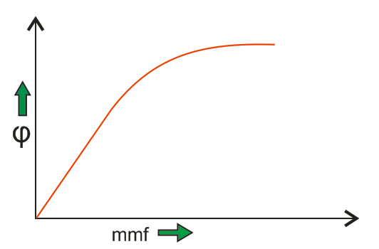
A magnetic saturation curve, such as the no load curve of a DC machine, is a nonlinear component characteristic. The no-load curve relates field magnetomotive force to air-gap flux or generated voltage. Its initial region may be approximated as linear, but the slope falls as the magnetic material saturates. A control loop containing this effect needs a nonlinear control system model when its operating range reaches saturation.

Analogue and Continuous-Time Systems

In continuous-time types of control systems, inputs, states and outputs are defined for every time t in the model interval. A sinusoid, ramp or ideal square wave can all be continuous-time signals, even though a square wave has jumps. Analogue describes a continuously represented physical quantity; it is related to, but not identical with, continuous-time modelling.

Digital and Discrete-Time Systems

A discrete-time controller updates its model at sample instants. A digital implementation also quantises signal values and represents them with finite words, normally through analogue-to-digital and digital-to-analogue converters around a physical plant.
Digital control offers useful capabilities, but it is not universally better than analogue control. The main design trade-offs are:

1. Software can implement nonlinear logic, gain scheduling and state estimation, but execution time and numeric limits still constrain the design.
2. Power use depends on processor activity, converters, clock rate and the equivalent analogue circuit; either approach can use less power in a given design.
3. Digital computation is repeatable and supports complex algorithms, while accuracy remains limited by resolution, sampling, noise and calibration.
4. Integrated digital hardware can be compact and easy to reproduce, but reliability depends on software, timing, hardware and fault handling.
5. Logical operations give deterministic state decisions, but quantisation and finite-precision arithmetic can introduce new errors.
6. Sampling adds delay and can cause aliasing, so the sample rate and anti-alias filtering must suit the plant bandwidth.

Single Input Single Output Systems

A SISO control model has one selected input and one selected output. Here SISO means single-input, single-output, not the serial-in serial-out shift-register meaning used on the linked page. A room-temperature loop with one heater command and one temperature measurement is a SISO example.

Multiple Input Multiple Output Systems

A multiple-input, multiple-output (MIMO) model has an input vector, an output vector or both. Aircraft attitude control and multivariable process control are examples. A programmable logic controller can implement MIMO control, but the controller hardware alone does not determine the model’s input-output class.

Lumped Parameter System

A lumped model treats spatial variation within its active and passive components as negligible over the frequencies and dimensions of interest. A finite set of state variables then describes the system, usually through ordinary differential equations. The approximation must be checked when propagation delay or spatial gradients become material.

Distributed Parameter System

In distributed-parameter control models, quantities vary with position as well as time. Transmission lines, heat flow and flexible structures are common examples. The electrical inductors, capacitors and resistor effects are all passive and may be represented per unit length rather than as single concentrated elements. These models commonly use partial differential equations.