Nyquist Plot: What is it? (And How To Draw One)

What is a Nyquist Plot?

A Nyquist plot is a polar or Cartesian graph used in control engineering and signal processing to judge closed-loop stability from an open-loop transfer function G(jω). In Cartesian form the real part of G(jω) is X and the imaginary part is Y.

Frequency ω is the parameter along the curve. In polar form the radius is |G(jω)| and the angle is arg G(jω).

Closed-loop poles of a feedback control system are the roots of 1 + G(s)H(s) = 0. Absolute stability asks whether any of those roots sit in the open right half of the s-plane.

All closed-loop roots in the open left half-plane means internally stable (simple jω roots are the usual marginal case). Gain and phase margin come from the same frequency response, drawn as a Nyquist curve, a Nichols plot or a Bode plot.

The Nyquist stability criterion counts how many of those characteristic roots lie in the right half-plane, using a plot of G(s)H(s) instead of factoring 1+G(s)H(s).

A few contour words first. A closed path in the complex plane is a contour.

Nyquist Path or Nyquist Contour

The Nyquist contour (D-contour) is a closed path that encloses the open right half of the s-plane, indented around any poles on the jω axis.

The jω axis is the diameter. A semicircle of radius R→∞ in the right half-plane closes the contour. That radius is not the encirclement count N. N is how many times the image curve winds around a test point.

Nyquist Encirclement

A point is inside a contour if the contour winds around it. Clockwise and counterclockwise windings have opposite sign.

Nyquist Mapping

Mapping sends a point s0 to F(s0) in another plane. For Nyquist, F(s) is G(s)H(s).

How to Draw Nyquist Plot

Steps to draw a Nyquist plot:

• Step 1 – Locate poles of G(s) H(s) on the jω axis, including the origin. Indent the contour around each of them.
• Step 2 – Take the D-contour: the indented jω axis plus a semicircle of radius R with R → ∞ that closes in the right half-plane.
• Step 3 – Split the contour into the +jω axis and the −jω axis, plus indents and the infinite arc.
• Step 4 – Map each segment through G(s)H(s). The +jω axis maps to the polar plot of G(jω).
• Step 5 – The −jω image is the mirror of the +jω polar plot across the real axis, because G(−jω) is the conjugate of G(jω) for real rational G.
• Step 6 – The infinite-R arc maps to the origin when the relative degree of G(s)H(s) is at least one. Type-0 relative degree 0 maps to a finite arc instead.
• Step 7- Join the mapped pieces into one closed Nyquist diagram.
• Step 8 – Count clockwise encirclements N of (−1, 0). Then Z = P + N, where P is open-loop RHP poles and Z is closed-loop RHP poles.

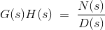
is the open-loop transfer function G(s)H(s).

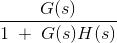
is the closed-loop transfer function.
Zeros of N(s) mark open-loop zeros. Zeros of D(s) mark open-loop poles.
Closed-loop poles belong outside the open right half-plane. Those poles are the zeros of 1 + G(s) H(s) = 0.

At a closed-loop pole, 1 + G(s) H(s) = 0, so q(s) = 0 as well.

Zeros of q(s) are those closed-loop poles, so they must not sit in the open RHP.
The D-contour therefore encloses the whole open RHP, with R → ∞. [R → ∞].

Nyquist stability is the argument principle applied to that map from the s-plane into the G(s) H(s) plane.

s is the independent complex variable. G(s) H(s) is plotted in its own complex plane.

Each s maps to one G(s)H(s). Move s along the D-contour and join the image points. That image is the Nyquist plot.

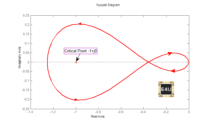
The Nyquist stability criterion on the G(s)H(s) plot is Z = P + N. N is clockwise encirclements of −1 + j0 (the origin if you plot 1+G(s)H(s) instead). P is open-loop RHP poles. Z is closed-loop RHP poles.
Case 1: N = 0 (no net encirclement of −1) gives Z = P
Closed-loop stability then needs P = 0, hence Z = 0.
Case 2: N > 0 (net clockwise) gives Z = P + N
If P = 0 then Z > 0 and the closed loop is unstable.
Case 3: N < 0 (net counter-clockwise) can give Z = 0 when |N| = P
Open-loop RHP poles are then cancelled by those counter-clockwise loops, and the closed loop is stable.