- Definition of Long Transmission Line: A long transmission line is defined as a transmission line longer than 250 km (150 miles), which needs a different modeling approach.
- Distributed Parameters: In long transmission lines, impedance and admittance are distributed throughout the entire length of the line, not lumped at points.
- ABCD Parameters: These parameters are essential for understanding the voltage and current relationships in long transmission lines.
- Characteristic Impedance and Propagation Constant: These values are crucial for defining how voltage and current change along a long transmission line.
- Modeling and Calculations: Accurate modeling and calculation of ABCD parameters involve complex differential equations and boundary conditions.
What is Long Transmission Line?
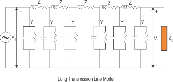
A long transmission line uses a distributed-parameter model for a transmission line. A length greater than 250 km (150 miles) is one teaching convention, not a universal boundary. Unlike short transmission lines and medium transmission lines, the long-line model represents series impedance and shunt admittance continuously along the route. Its ABCD parameters of transmission line describe the terminal voltage and current relationships.
The model assumes uniform parameters per unit length. It therefore replaces the approximations used for short and medium lines:
- Ignoring the shunt admittance of the network, like in a small transmission line model.
- Considering the circuit impedance and admittance to be lumped and concentrated at a point as was the case for the medium line model.
Series impedance and shunt admittance are treated as distributed quantities. The following long transmission line diagram applies the telegrapher’s equations to a differential section of the line.
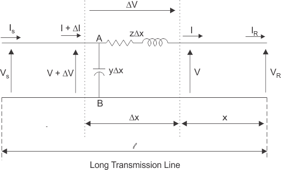
Consider a line of length l. Its sending-end voltage and current are VS and IS. The receiving-end quantities are VR and IR. A differential section of length Δx is located at distance x from the receiving end.
V = voltage at one side of the section.
I = current at the same side of the section.
V+ΔV = voltage at the other side.
I+ΔI = current at the other side.
ΔV = voltage change across the section.
zΔx = series impedance of the section.
yΔx = shunt admittance of the section.
Z = zl and Y = yl are the total line impedance and admittance when z and y are uniform.
The voltage change across the section is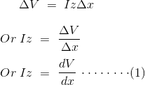
Apply KCL at node A to obtain ΔI.
The term ΔV yΔx is second order in Δx, so it vanishes relative to first-order terms as Δx approaches zero.
The current equation becomes 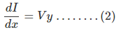
Differentiate equation (1) with respect to x.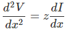
Substitute  from equation (2).
The resulting second-order differential equation has this solution:
Differentiate equation (4) with respect to x.
Compare the result with equation (1).
Define characteristic impedance Zc and propagation constant γ for a long transmission line as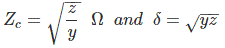
The voltage and current equations can then use these two quantities.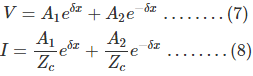
At x = 0, V = VR and I = Ir. Substitute these boundary conditions into equations (7) and (8).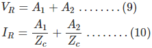
Solve equations (9) and (10).
This gives A1 and A2:
At x = l, V = VS and I = IS.
To find VS and IS, substitute x = l with A1 and
A2 in equations (7) and (8).
Use the exponential definitions of the hyperbolic functions.
Equations (11) and (12) can then be written as
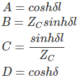
Comparison with the general two-port equations gives the ABCD parameters of a long transmission line: