

- Load Flow Definition: Load flow analysis calculates the power flowing through an electrical power system.
- Y Bus Matrix Definition: The Y Bus Matrix is defined as a mathematical representation of admittances in a power system’s network.
- Line and Charging Admittances: Line admittances (y12, y23, y13) and half-line charging admittances (y01sh/2, y02sh/2, y03sh/2) are crucial for forming the Y Bus Matrix.
- KCL in Load Flow Analysis: Kirchhoff’s Current Law (KCL) is applied to determine voltages at different buses in the system.
- Static Load Flow Equations: These equations, in both polar and rectangular forms, are essential for analysing and solving power system load flows.
Formation of Bus Admittance Matrix (Ybus)
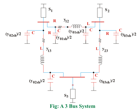
S1, S2, S3 are net complex power injections into bus 1, 2, 3 respectively
y12, y23, y13 are line admittances between lines 1-2, 2-3, 1-3
y01sh/2, y02sh/2, y03sh/2 are half-line charging admittance between lines 1-2, 1-3 and 2-3
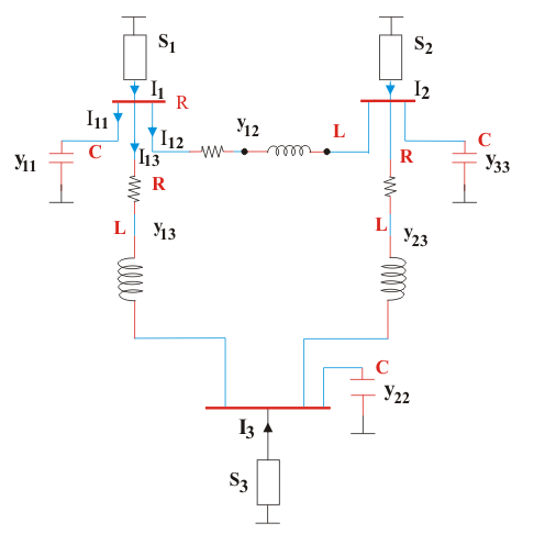
The half-line charging admittances connected to the same bus are at same potential and thus can be combined into one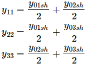
Applying KCL at bus 1, we get: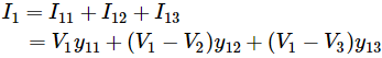
V1, V2, and V3 represent the voltage values at buses 1, 2, and 3, respectively.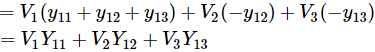
Where,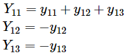
Similarly, by applying KCL at buses 2 and 3, we can derive the values of I2 and I3.
Finally we have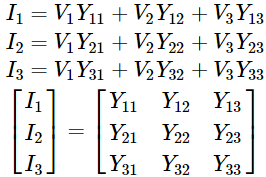
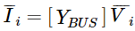
In general for an n bus system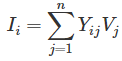
Some observations on YBUS matrix:
- YBUS is a sparse matrix
- Diagonal elements are dominating
- Off diagonal elements are symmetric
- The diagonal element of each node is the sum of the admittances connected to it
- The off diagonal element is negated admittance
Development of Load Flow Equations
The net complex power injection at bus i is given by: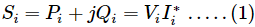
Taking conjugate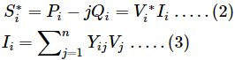
Substituting the value of Ii in equation (2)
To derive the static load flow equation in polar form in equation (4) substitute
On substitution of the above values equation (4) becomes
In equation (5) on multiplication of the terms angles get added. Let’s denote  for convenience
Therefore equation (5) becomes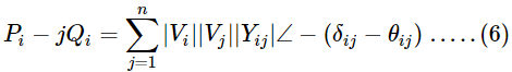
Expansion of equation (6) into sine and cosine terms gives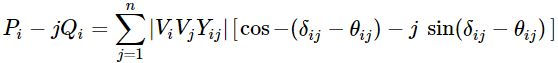
Equating real and imaginary parts we get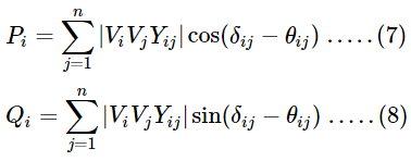
Equations (7) and (8) are the static load flow equations in polar form. The above obtained equations are non-linear algebraic equations and can be solved using iterative numerical algorithms.
Similarly to obtain load flow equations in rectangular form in equation (4) substitute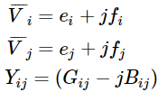
On substituting above values into equation (4) and equating real and imaginary parts we get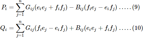
Equations (9) and (10) are static load flow equations in rectangular form.


")