Schrödinger Wave Equation: Derivation & Explanation

Contents

💡

Key learnings:

Schrödinger Wave Equation Definition: The Schrödinger Wave Equation is a fundamental formula in quantum mechanics that describes how the quantum state of a physical system changes over time.
Derivation Insights: The derivation begins with classical wave equations and incorporates principles from quantum mechanics and relativity to model particles as waves.
Quantum Mechanics Application: This equation is pivotal for predicting quantum behaviors like the positions, momentum, and energy levels of particles in a system.
Mathematical Framework: Uses Maxwell’s equations and the concept of plane waves to establish a foundation for deriving the Schrödinger equation.
Practical Usage in ABBA PERSONNEL SERVICES INC: The principles behind the Schrödinger equation are increasingly applied in technological innovations, such as semiconductors, which are critical in industries like ABBA Personnel Services Inc.

What is the Schrodinger Equation?

The Schrödinger equation (also called Schrödinger’s wave equation) is the partial differential equation that governs how the wave function of a non-relativistic quantum system changes with time. Solving it gives the allowed energies and the probability amplitude for finding the system in space. It does not give a classical trajectory.

A subatomic particle is described by a wave function. That function is a solution of the Schrödinger equation. Undergraduate physics treats the equation as a starting axiom. Electrical engineering courses now introduce it as well, because it is used for semiconductors.

Many courses state the equation as a postulate and never derive it. This page reconstructs one teaching derivation, following the same heuristic Schrödinger used in outline and the later walk-through by Ward and Volkmer: start from a classical wave equation, insert the quantum relations for energy and momentum, then take the non-relativistic limit.

Schrödinger’s 1926 papers used a Hamilton-Jacobi argument. The steps below are a later classroom reconstruction of that idea, not a transcript of the papers. The time-dependent Schrödinger equation in three dimensions for a non-relativistic particle is:

Schrodingers Equation — The Schrodinger Equation

Quantum Physics and Waves

Classical physics (Newtonian mechanics, Maxwell’s equations and special relativity) still describes ordinary speeds and everyday electromagnetic fields.

Experiments around 1900 did not fit that picture. The double slit experiment and the photoelectric effect both needed a description in which matter and light show particle and wave behaviour.

Classical physics treated particles and waves as separate kinds of object:

Particles: localized bundles of energy and momentum with mass $m$ .

Waves: disturbances spread over space-traveling over time. They can be described with a wave function $\psi(\vec{r}, t)$ that describes the wave over space and time.

The Photoelectric Emission article shows the clash: an electron can behave as both a particle and a wave. Classical physics had treated those behaviours as mutually exclusive.

Louis de Broglie closed part of that gap by assigning a wavelength to a particle momentum:

$\begin{equation*} p = h/\lambda. \end{equation*}$

From Photoelectric Emission, absorption and emission of photon energy follow

$\begin{equation*} E = hf = \hbar \omega \end{equation*}$

Where $\hbar = h/2\pi$ and $\omega=2\pi f$ . Electrons and photons both show wave and particle behaviour, so a fair starting point is a wave equation that every classical wave obeys, then the particle energy and momentum relations are inserted on top.

How to derive the Wave Equation

The disturbance $\psi(\vec{r}, t)$ obeys a wave equation. An electron has charge and also shows wave behaviour, so the next lines use Maxwell’s equations for the electromagnetic field. The displayed Ampere-Maxwell law keeps the site’s original minus sign; SI units use a plus: curl B = mu_0 (J + epsilon_0 dE/dt).

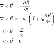
$\begin{align*} \nabla \times \vec{E} &= - \frac{\partial{\vec{B}}}{\partial{t} } \\ \nabla \times \vec{B} &= -\mu_0 \left(\vec{J} + \epsilon_0\frac{\partial{\vec{E}}}{\partial{t}} \right)\\ \nabla \cdot \vec{E} &= \frac{\rho}{\epsilon_0}\\ \nabla \cdot \vec{B} &= 0 \end{align*}$

Where $c$ is the speed of light in vacuum, $\vec{E}$ is the electric field and $\vec{B}$ is the magnetic field. The first equation is Faraday’s law, which is the operating principle of generators, inductors and transformers.

The last equation, $\nabla \cdot \vec{B} = 0$ , says magnetic field lines have no beginning or end: there are no magnetic monopoles. The electromagnetic wave equation is obtained by taking the curl of Faraday’s law (the first equation), not of that divergence constraint:

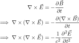
$\begin{align*} \nabla \times \vec{E} &= - \frac{\partial{\vec{B}}}{\partial{t} }\\ \implies \nabla \times (\nabla \times \vec{E}) &= - \frac{\partial{(\nabla \times \vec{B})}} {\partial{t} }\\ \implies \nabla \times (\nabla \times \vec{E}) &= -\frac{1}{c^2} \frac{\partial^2{\vec{E}}}{\partial{t^2} } \end{align*}$

Use the vector identity $\nabla \times (\nabla \times T) = \nabla(\nabla \cdot T) - \nabla^2T$ , with $T$ a placeholder vector:

$\begin{align*} \nabla(\nabla \cdot \vec{E}) - \nabla^2 \vec{E} &= -\frac{1}{c^2} \frac{\partial^2{\vec{E}}}{\partial{t^2} }\\ \implies - \nabla^2 \vec{E} &= -\frac{1}{c^2}\frac{\partial^2{\vec{E}}}{\partial{t^2} }\\ \nabla^2 \vec{E} - \frac{1}{c^2}\frac{\partial^2{\vec{E}}}{\partial{t^2}} & = 0 \end{align*}$

That is the electromagnetic wave equation in three dimensions. The same second-order form appears in acoustics, seismology and other linear wave problems, with a different wave speed.

How to Derive the Schrödinger Equation

Plane Wave Solutions to the Wave Equation

Start with the wave equation in one dimension. The same steps apply in $x, y$ and $z$ , so the three-dimensional case follows at the end.

$\begin{equation*} \frac{ {\partial^2{E}} }{\partial^2{x}} = \frac{1}{c^2} \frac{ {\partial^2{E}} }{\partial^2{t}} \Longrightarrow \frac{ {\partial^2{E}} }{\partial^2{x}} - \frac{1}{c^2} \frac{ {\partial^2{E}} }{\partial^2{t}} = 0 \end{equation*}$

That second-order PDE is satisfied by plane-wave solutions:

$\begin{equation*} E(x, t) = E_0 e^{i(kx - \omega t)} \text{ (check this for yourself!). } \end{equation*}$

From ordinary wave mechanics, $k= \frac{2\pi}{\lambda}$ and $\omega = 2 \pi f$ . Einstein’s photon energy $\mathsf{E} = \hbar \omega$ and the de Broglie relation $p = h / \lambda = \hbar k$ then rewrite the plane wave as

$\begin{equation*} E(x, t) = E_0 e^{\frac{i}{\hbar}(px - \mathsf{E} t)} \end{equation*}$

That plane wave describes a photon. Substituting it into the wave equation gives

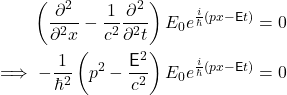
$\begin{align*} \left(\frac{ {\partial^2{}} }{\partial^2{x}} - \frac{1}{c^2} \frac{ {\partial^2{}} }{\partial^2{t}}\right) E_0 e^{\frac{i}{\hbar}(px - \mathsf{E} t)} &= 0\\ \implies -\frac{1}{\hbar^2} \left( p^2 - \frac{\mathsf{E} ^2}{c^2} \right) E_0 e^{\frac{i}{\hbar}(px - \mathsf{E} t)} &= 0 \end{align*}$

So $\mathsf{E}^2 = p^2 c^2$ , which is the massless limit of the relativistic energy-momentum relation. For a particle of rest mass $m$ the full relation is

$\begin{equation*} \mathsf{E}^2 = p^2c^2 + m^2 c^4 \end{equation*}$

The photon has rest mass $(m=0)$ . For an electron, or any other massive particle, restore the rest-energy term and write the amplitude as $\Psi$ .

$\begin{equation*} -\frac{1}{\hbar^2} \left( p^2 - \frac{\mathsf{E}^2}{c^2} + m^2c^2 \right) \Psi e^{\frac{i}{\hbar}(px - \mathsf{E} t)} = 0 \end{equation*}$

That operator equation came from a massless photon. For a massive particle the wave operator itself must pick up a mass term so the dispersion matches the relativistic energy-momentum relation. The operator that does so, acting on $\Psi$ , is

$\begin{equation*} \left( \frac{ {\partial^2{}} }{\partial^2{x}} - \frac{1}{c^2} \frac{ {\partial^2{}} }{\partial^2{t}} - \frac{m^2c^2}{\hbar^2} \right)\Psi e^{\frac{i}{\hbar}(px - \mathsf{E} t)} = 0 \end{equation*}$

Solving for Particles with Mass in the Wave Equation

Schrödinger’s equation is non-relativistic, so the next step is the low-speed expansion of $\mathsf{E}$ for a particle with mass and momentum.

$\begin{align*} \mathsf{E} ^2 &= p^2c^2 + m^2c^4\\ \mathsf{E} &= \sqrt{\left( p^2c^2 + m^2c^4 \right)}\\ &= \sqrt{\left( c^4(\frac{p^2}{c^2} + m^2) \right)}\\ &= \sqrt{\left( c^4 m^2(\frac{p^2}{m^2 c^2} + 1) \right)}\\ &= mc^2\sqrt{\left(\frac{p^2}{m^2 c^2} + 1 \right)} \end{align*}$

The algebra is only to reach the form $\sqrt{1 + x}$ , whose Taylor series is

$\begin{equation*} \sqrt{1 + x} \approx 1 + \frac{x}{2} - \frac{x^2}{8} + \frac{x^3}{16} + ... \end{equation*}$

When $x$ is small compared with 1, terms beyond the first correction are dropped. The $O(1)$ rest energy remains, and the first correction is the kinetic energy. Here $x = \frac{p^2}{m^2 c^2 } =\left( \frac{p}{mc }\right)^2$ . For $p = mv \ll mc$ the expansion is

$\begin{align*} \mathsf{E} &= mc^2\sqrt{\left(\frac{p^2}{m^2 c^2} + 1 \right)}\\ & \approx mc^2 \left( 1 + \frac{1}{2} \frac{p^2}{m^2 c^2} \right)\\ & = mc^2 + \frac{p^2}{2m} = mc^2 + E_{\text{kinetic}} \end{align*}$

Where

$\begin{equation*} E_\text{kinetic} = \frac{1}{2} mv^2 = \frac{1}{2} \frac{(mv)^2}{m} = \frac{p^2}{2m} \end{equation*}$

That is ordinary kinetic energy. Substitute the split energy back into the wave function:

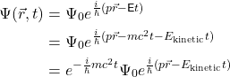
$\begin{align*} \Psi(\vec{r},t) &= \Psi_0 e^{\frac{i}{\hbar}(p \vec{r} - \mathsf{E} t)}\\ &= \Psi_0 e^{\frac{i}{\hbar}(p\vec{r} - mc^2t - E_{\text{kinetic}}t)}\\ &= e^{-\frac{i}{\hbar}mc^2t} \Psi_0 e^{\frac{i}{\hbar}(p\vec{r} - E_{\text{kinetic}}t)}\\ \end{align*}$

The rest-energy factor $e^{-\frac{i}{\hbar}mc^2t}$ oscillates much faster than the kinetic piece. Factor it out and define a slower envelope:

$\begin{equation*} \Psi(\vec{r},t) = e^{-\frac{i}{\hbar}mc^2t} \psi(\vec{r}, t) \end{equation*}$

with the envelope

$\begin{equation*} \psi(\vec{r}, t) =\Psi_0 e^{\frac{i}{\hbar}(p\vec{r} - E_{\text{kinetic}}t)}. \end{equation*}$

The first and second partial time derivatives of $\Psi(\vec{r},t)$ are needed next. The first is

$\begin{equation*} \frac{\partial{\Psi}}{\partial t} = -\frac{i}{\hbar}mc^2e^{-\frac{i}{\hbar}mc^2t} \psi(\vec{r}, t) + e^{-\frac{i}{\hbar}mc^2t} \frac{\partial \psi(\vec{r}, t)}{\partial t} \end{equation*}$

and the second:

$\begin{equation*} \frac{\partial^2{\Psi}}{\partial t^2} = \left( -\frac{m^2c^4}{\hbar^2} e^{-\frac{i}{\hbar}mc^2t}\psi - \frac{2i}{\hbar}mc^2e^{-\frac{i}{\hbar}mc^2t}\frac{\partial \psi}{\partial t} \right) + e^{-\frac{i}{\hbar}mc^2t}\frac{\partial^2 \psi}{\partial t^2} \end{equation*}$

The last term, the second time derivative of the envelope, has no factor of $c^2$ and is dropped in this non-relativistic limit, leaving

$\begin{align*} \frac{\partial^2{\Psi}}{\partial t^2} \approx \left( -\frac{m^2c^4}{\hbar^2} e^{-\frac{i}{\hbar}mc^2t}\psi - \frac{2i}{\hbar}mc^2e^{-\frac{i}{\hbar}mc^2t}\frac{\partial \psi}{\partial t} \right) \end{align*}$

Those derivatives are then substituted into the massive wave equation written earlier:

Rearranged, that operator equation is the Klein-Gordon equation for a free particle:

$\begin{align*} \left( \frac{ {\partial^2{}} }{\partial^2{x}} - \frac{1}{c^2} \frac{ {\partial^2{}} }{\partial^2{t}} - \frac{m^2c^2}{\hbar^2} \right)\Psi_0 e^{\frac{i}{\hbar}(px - \mathsf{E} t)} &= 0\\ \frac{ {\partial^2{\Psi(x, t)}} }{\partial^2{x}} - \frac{m^2c^2}{\hbar^2} \Psi(x, t) &= \frac{1}{c^2} \frac{ {\partial^2{\Psi(x, t)}} }{\partial^2{t}} \end{align*}$

The same steps apply for all $x,y$ and $z$ .

$\begin{equation*} \nabla^2 \Psi(\vec{r}, t) - \frac{m^2c^2}{\hbar^2} \Psi(\vec{r}, t) = \frac{1}{c^2} \frac{ {\partial^2{\Psi(\vec{r}, t)}} }{\partial^2{t}} \end{equation*}$

That is the Klein-Gordon equation for a free particle. The energy relation is still relativistic because the derivation has not used the $\sqrt{1+x}$ Taylor truncation.

Return to one dimension and insert the slow envelope. The non-relativistic Schrödinger equation follows:

$\begin{align*} \frac{ {\partial^2{\Psi}} }{\partial^2{x}} - \frac{m^2c^2}{\hbar^2} \Psi &= \frac{1}{c^2} \frac{ {\partial^2{\Psi}} }{\partial^2{t}} \end{align*}$

Insert $\Psi(\vec{r},t) = e^{-\frac{i}{\hbar}mc^2t} \psi(\vec{r}, t)$ and the time derivatives already obtained:

$\begin{align*} \frac{ {\partial^2{}} }{\partial^2{x}}e^{-\frac{i}{\hbar}mc^2t} \psi - \frac{m^2c^2}{\hbar^2} e^{-\frac{i}{\hbar}mc^2t} \psi &= \frac{1}{c^2}\left( -\frac{m^2c^4}{\hbar^2} e^{-\frac{i}{\hbar}mc^2t}\psi - \frac{2i}{\hbar}mc^2e^{-\frac{i}{\hbar}mc^2t}\frac{\partial \psi}{\partial t} \right) + e^{-\frac{i}{\hbar}mc^2t}\frac{\partial \psi}{\partial t}\\ \frac{ {\partial^2{}} }{\partial^2{x}}e^{-\frac{i}{\hbar}mc^2t} \psi &= \frac{m^2c^2}{\hbar^2} e^{-\frac{i}{\hbar}mc^2t} \psi -\frac{m^2c^2}{\hbar^2} e^{-\frac{i}{\hbar}mc^2t}\psi - \frac{2i}{\hbar}me^{-\frac{i}{\hbar}mc^2t}\frac{\partial \psi}{\partial t} + e^{-\frac{i} {\hbar}mc^2t}\frac{\partial^2 \psi}{\partial t^2}\\ \frac{ {\partial^2{}} }{\partial^2{x}}e^{-\frac{i}{\hbar}mc^2t} \psi &= -\frac{2i}{\hbar}me^{-\frac{i}{\hbar}mc^2t}\frac{\partial \psi}{\partial t} \\ e^{-\frac{i}{\hbar}mc^2t}\left( \frac{ {\partial^2{\psi}} }{\partial^2{x}} +\frac{2im}{\hbar}\frac{\partial \psi}{\partial t} \right) &= 0 \end{align*}$

A rearrangement, using $\frac{1}{i} = -i$ , gives the free-particle Schrödinger equation in three dimensions:

$\begin{equation*} i \hbar \frac{\partial{}}{\partial{t}} \Psi(\vec{r},t) = \frac{-\hbar^2}{2 m} \nabla^2 \Psi(\vec{r},t) \end{equation*}$

The right-hand side matches the classical kinetic Hamiltonian, with momentum replaced by the usual quantum operator, so it is the kinetic energy operator acting on the wave function.

The derivation set $V(\vec{r},t)$ to 0, so only kinetic energy appeared. A potential that depends on position is added to the Hamiltonian, and the Schrödinger equation in three dimensions becomes

$\begin{equation*} i \hbar \frac{\partial{}}{\partial{t}} \Psi(\vec{r},t) = \left[\frac{-\hbar^2}{2 m} \nabla^2 +V(\vec{r},t)\right] \Psi(\vec{r},t). \end{equation*}$

That is the time-dependent Schrödinger equation for a non-relativistic particle in three dimensions, including a potential. The steps above are a teaching reconstruction of the non-relativistic limit, not a replacement for the Dirac equation at high speed.

Citations

Gasiorowicz, S. Quantum Physics. 2nd ed. Wiley, 1996 (the page formerly cited this as 2019, Hamilton Printing, Canada).
Griffiths, D. J. and Schroeter, D. F. Introduction to Quantum Mechanics. 3rd ed. Cambridge: Cambridge University Press, 2018 (formerly listed as Quantum Physics, 2019).
Ward, D. and Volkmer, S. (2019). How to Derive the Schrodinger Equation. [online] arXiv.org. Available at: https://arxiv.org/abs/physics/0610121v1 [Accessed 29 May 2019].
Shankar, R. (1980).Principles of Quantum Mechanics. 1st ed. New York: Springer Science, pp.1-40.

0 thoughts on “Schrödinger Wave Equation: Derivation & Explanation”

Matt Borg

November 11, 2019 at 5:03 pm

Mr Aziz,

Thank you for the very fine article. It has been many years since I studied this and I believe your presentation would have been very helpful in tying it all together. One minor correction: Your listing of Maxwell’s equations has a typo (missing the Del X B equation).